Person assessment with PPass, also for eRm models
Manuel Reif
Source:vignettes/ppass_erm.Rmd
ppass_erm.RmdPPass() (Person
Parameter assessment) estimates the
abilities, computes the person fit and returns both in one table,
together with the other person variables. It accepts
- a data.frame (or matrix) with item responses, together with known item parameters, or
- a model fitted with the eRm package: the Rasch model, the linear logistic test model, the rating scale model, the partial credit model and their linear versions, also with several time points and groups.
Data with item parameters
fourpl_df contains an id, the sex and the responses of
60 persons to 12 items of a 3PL test. items names the item
columns (positions or names); all other columns are kept as person
variables. mod chooses the model, and the item parameters
must match it.
library(PP)
data(fourpl_df)
res <- PPass(fourpl_df, items = 3:14,
             thres = attr(fourpl_df, "diffpar"), slopes = attr(fourpl_df, "slopes"),
             lowerA = attr(fourpl_df, "lowerA"))
res
#> Person assessment: 60 persons, 12 items
#> Model: 3PL model | WLE estimates
#> Status: 60 ok
#> Person fit: lz, lzstar, infit, outfit
#> Flagged (|lzstar| > 1.96): 4 persons
#>
#>         id sex estimate    SE status     lz lzstar infit    in_t outfit   ou_t
#> 1  LVL0694   w   -0.936 0.767     ok  1.019  1.026 0.692 -1.0907 0.5342 -0.866
#> 2  BBU1225   w    1.811 1.022     ok  1.101  1.149 0.377 -1.5365 0.2061 -0.526
#> 3  MJN2028   w    0.969 0.987     ok  1.270  1.324 0.288 -1.7568 0.2011 -1.204
#> 4  TSU0771   m    1.224 1.008     ok -1.039 -1.157 1.487  0.9781 1.9539  1.107
#> 5  XDS0698   w    0.252 0.925     ok  1.187  1.224 0.436 -1.3918 0.3219 -1.257
#> 6  BOS1292   w   -4.730 2.118     ok  0.998  0.637 0.108 -1.5050 0.0884 -1.196
#> 7  KFF1422   w    2.618 1.016     ok  0.545  0.580 0.765 -0.4927 0.3216  0.181
#> 8  DCQ0198   w    1.232 1.008     ok -1.099 -1.221 1.480  0.9681 2.2503  1.295
#> 9  FTT1492   w   -2.377 0.913     ok  0.182  0.103 0.973  0.0586 0.7565 -0.157
#> 10 GCP0645   m   -0.400 0.802     ok  0.922  0.948 0.678 -0.8861 0.5105 -0.932
#> ... 50 more persons
#> Not shown: lz_unst, in_chisq, in_df, in_pv, ou_chisq, ou_df, ou_pv
By default, PPass() computes WLE estimates and all four
person fit statistics (lz, lz*, infit and outfit). Other arguments of
PP_4pl(), PP_gpcm() and PPall()
can be passed on, e.g. type = "mle" or a prior for
type = "map". summary() shows the distribution
of the estimates, the person fit and the persons flagged by lz*
(two-sided, as in the summary of Pfit()):
s <- summary(res)
#> Person assessment: 60 persons, 12 items
#> Model: 3PL model | WLE estimates
#> Status: 60 ok
#> Person fit: lz, lzstar, infit, outfit
#> Flagged (|lzstar| > 1.96): 4 persons
#>
#> Estimates (status ok):
#>    Min. 1st Qu.  Median    Mean 3rd Qu.    Max.
#>  -4.730  -1.278  -0.339  -0.313   0.969   3.624
#>
#> Person fit:
#>  statistic  n   mean    sd     min  max flagged
#>         lz 60  0.245 1.012 -3.0334 1.33       3
#>     lzstar 60  0.192 1.093 -3.2532 1.34       4
#>      infit 60  0.870 0.430  0.1080 2.13      NA
#>       in_t 60 -0.292 1.013 -1.7568 2.28       2
#>     outfit 60  0.853 0.828  0.0884 4.29      NA
#>       ou_t 60 -0.163 0.980 -1.3185 3.01       3
#>
#> Flagged persons (lzstar):
#>  person      id sex estimate lzstar
#>      26 HBH0927   m    -0.57  -3.25
#>      60 RWQ0486   w    -2.16  -3.07
#>      43 WUS0752   w     0.78  -3.04
#>      39 UHY1090   m     2.88  -2.07
plot() shows the person fit map: lz* against the
estimate, with the critical values of summary() and the
flagged persons labelled, here by their id.
which = "precision" shows the measurement precision of the
test and which = "profile" the answers of single persons
(see ?"pp-plots").
plot(res, label = "id")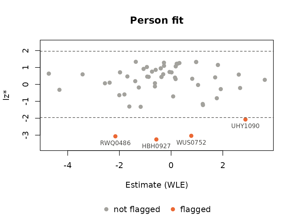
The result is a data.frame. It can be filtered, merged or written to
a file like any other data.frame; as.data.frame() drops the
extra information.
res[res$sex == "w" & res$status == "ok", c("id", "estimate", "SE", "lzstar")][1:5, ]
#>        id estimate    SE lzstar
#> 1 LVL0694   -0.936 0.767  1.026
#> 2 BBU1225    1.811 1.022  1.149
#> 3 MJN2028    0.969 0.987  1.324
#> 5 XDS0698    0.252 0.925  1.224
#> 6 BOS1292   -4.730 2.118  0.637
knitr::kable(head(as.data.frame(res)[, c("id", "sex", "estimate", "SE", "lzstar", "infit")]),
digits = 3)| id | sex | estimate | SE | lzstar | infit |
|---|---|---|---|---|---|
| LVL0694 | w | -0.936 | 0.767 | 1.026 | 0.692 |
| BBU1225 | w | 1.811 | 1.022 | 1.149 | 0.377 |
| MJN2028 | w | 0.969 | 0.987 | 1.324 | 0.288 |
| TSU0771 | m | 1.224 | 1.008 | -1.157 | 1.487 |
| XDS0698 | w | 0.252 | 0.925 | 1.224 | 0.436 |
| BOS1292 | w | -4.730 | 2.118 | 0.637 | 0.108 |
JKpp() and PV() work directly on the
result, without estimating again:
head(JKpp(res)$estimates)
#>     estimate        SE  L excluded status
#> 1 -0.9723726 0.6735435 12        0     ok
#> 2  1.8740917 0.6208916 12        0     ok
#> 3  1.0570466 0.4916653 12        0     ok
#> 4  1.5539111 1.6822352 12        0     ok
#> 5  0.3442215 0.5400380 11        0     ok
#> 6 -5.8298151 0.5859734 12        0     ok
The model follows from the item parameters: here slopes
and lowerA make it a 3PL model. A threshold matrix with
several thresholds per item gives the PCM (all slopes 1) or the GPCM;
together with lowerA or upperA it gives a test
with both dichotomous (4PL) and polytomous (GPCM) items, estimated with
PPall().
Models fitted with eRm
eRm estimates item parameters by conditional maximum likelihood;
eRm::person.parameter() then gives maximum likelihood
estimates of the abilities. PPass() takes the fitted object
and adds WLE, MAP, EAP and robust estimates, the person fit, the
jackknife and plausible values.
library(eRm)
rm1 <- RM(raschdat1)
res_rm <- PPass(rm1)
res_rm
#> Person assessment: 100 persons, 30 items
#> Model: Rasch model (eRm::RM) | WLE estimates
#> Status: 100 ok
#> Person fit: lz, lzstar, infit, outfit
#> Flagged (|lzstar| > 1.96): 4 persons
#>
#>    estimate    SE status        lz  lzstar infit     in_t outfit    ou_t
#> 1     -3.29 0.868     ok  0.411679  0.2080 0.722 -0.16277  0.478 -0.2043
#> 2     -2.72 0.688     ok  0.000319 -0.8777 0.946  0.07782  1.003  0.2821
#> 3     -2.33 0.596     ok  0.180246 -0.0421 0.954  0.03047  0.736 -0.2103
#> 4     -2.02 0.539     ok  0.518854  0.9215 0.845 -0.35622  0.661 -0.4994
#> 5     -2.02 0.539     ok  0.134508 -0.0476 0.952 -0.02333  0.857 -0.0800
#> 6     -2.02 0.539     ok -0.079114 -0.5862 1.034  0.21354  0.932  0.0643
#> 7     -1.76 0.499     ok  0.611982  1.0803 0.843 -0.47085  0.665 -0.6300
#> 8     -1.54 0.471     ok -0.229133 -0.6356 0.977 -0.00897  1.846  1.7622
#> 9     -1.54 0.471     ok  0.055611 -0.0814 1.029  0.19749  0.831 -0.2891
#> 10    -1.54 0.471     ok -0.081792 -0.3488 1.011  0.12597  1.023  0.1941
#> ... 90 more persons
#> Not shown: lz_unst, in_chisq, in_df, in_pv, ou_chisq, ou_df, ou_pv
The maximum likelihood estimates are the same as those of eRm:
res_mle <- PPass(rm1, type = "mle", fitindices = "lzstar")
pp <- person.parameter(rm1)
ok <- res_mle$status == "ok"
max(abs(res_mle$estimate[ok] - pp$theta.table[ok, "Person Parameter"]))
#> [1] 2.456019e-05
eRm stores the parameters of the item categories as easiness
parameters. PPass() converts them into PP thresholds, so
the eRm package is not even needed to run PPass() on a
saved object. Partial credit and rating scale models are estimated with
PP_gpcm(), with all slopes equal to 1:
set.seed(2751)
thres <- rbind(c(-2, -1.2, -0.5, 0), c(-1, 0.3, 1, 1.5), c(0.5, NA, NA, 2))
x <- sim_gpcm(thres = thres, alpha = 1, theta = rnorm(300))
res_pcm <- PPass(PCM(x), type = "map")
summary(res_pcm$estimate)
#>    Min. 1st Qu.  Median    Mean 3rd Qu.    Max.
#> -1.5928 -0.5035  0.1379  0.0808  0.4635  1.9687
With several time points (mpoints) and groups
(groupvec), every combination of item, time point and group
is a virtual item with its own parameters. A person answers the virtual
items of their group and gets one ability estimate across all time
points. eRm gives no person parameters for models with group contrasts;
PPass() does:
x2 <- sim_gpcm(thres = thres, alpha = 1, theta = rnorm(300, 0.5))
lpcm <- LPCM(cbind(x, x2), mpoints = 2, groupvec = rep(1:2, 150))
res_lpcm <- PPass(lpcm)
res_lpcm
#> Person assessment: 300 persons, 16 virtual items
#> Model: linear partial credit model (eRm::LPCM), 2 time points, 2 groups | WLE estimates
#> Status: 300 ok
#> Person fit: lz, lzstar, infit, outfit
#> Flagged (|lzstar| > 1.96): 7 persons
#>
#>    group estimate    SE status     lz lzstar infit   in_t outfit    ou_t
#> 1      1  -1.0074 0.496     ok  0.260  0.271 0.872 -0.140  0.845 -0.1578
#> 2      2  -0.3677 0.454     ok  0.218  0.220 0.833 -0.285  0.972  0.0761
#> 3      1   0.2085 0.453     ok -1.223 -1.260 1.284  0.736  1.256  0.6987
#> 4      2   1.0699 0.500     ok  1.077  1.404 0.328 -1.768  0.377 -1.3477
#> 5      1   0.0114 0.450     ok  1.326  1.328 0.334 -1.975  0.374 -1.8644
#> 6      2   0.4210 0.458     ok  0.444  0.463 0.618 -0.835  0.668 -0.7103
#> 7      1   0.0114 0.450     ok -0.654 -0.656 1.053  0.264  1.164  0.5115
#> 8      2   0.2201 0.453     ok  0.782  0.797 0.578 -0.982  0.562 -1.0909
#> 9      1  -0.3797 0.454     ok -1.543 -1.634 1.398  0.986  1.586  1.3135
#> 10     2   0.0231 0.450     ok  1.377  1.379 0.477 -1.368  0.478 -1.4254
#> ... 290 more persons
#> Not shown: lz_unst, in_chisq, in_df, in_pv, ou_chisq, ou_df, ou_pv
Plausible values need a prior, so they require an EAP or MAP
estimate, such as res_pcm above: