PP estimates person parameters (abilities) when the item parameters are already known, for example from an earlier calibration or an item bank. It is the right package if
- you have item responses of a group of persons,
- you have item parameters for these items, which are treated as fixed,
- the items follow the 1PL to 4PL model, the (generalized) partial credit model, or a mix of both,
and you want ability estimates (MLE, WLE, MAP, EAP or a robust estimate), jackknife estimates, plausible values or person fit statistics.
This vignette shows the estimation functions. Person fit is the topic
of vignette("intro_pfit"). Estimation and person fit in one
step and models fitted with the eRm package are shown in
vignette("ppass_erm").
A 3PL test
The data set fourpl_df contains the responses of 60
persons to 12 items, together with an id and the sex of each person. The
item parameters are attributes of the data set.
library(PP)
data(fourpl_df)
head(fourpl_df[, 1:7])
#>        id sex Item1 Item2 Item3 Item4 Item5
#> 1 LVL0694   w     1     1     1     1     0
#> 2 BBU1225   w     1     1     1     1     1
#> 3 MJN2028   w     1     1     1     1     1
#> 4 TSU0771   m     1     1     1     0     1
#> 5 XDS0698   w     1     1    NA     1     1
#> 6 BOS1292   w     0     0     0     0     0

diff_par  <- attr(fourpl_df, "diffpar")
slope_par <- attr(fourpl_df, "slopes")
low_par   <- attr(fourpl_df, "lowerA")
items <- as.matrix(fourpl_df[, -(1:2)])
PP_4pl() covers all dichotomous models. Which model is
used depends on the item parameters you supply: difficulties
(thres) alone give the 1PL model, adding
slopes gives the 2PL model, adding lowerA
gives the 3PL model, and adding upperA as well gives the
4PL model. Here the difficulties, slopes and lower asymptotes are known,
so the 3PL model is used.
res_mle <- PP_4pl(respm = items, thres = diff_par, slopes = slope_par, lowerA = low_par,
                  type = "mle")
#> Warning: 1 person(s) without a solution inside 'range' = c(-6, 6): the estimate
#> is set to the bound (status "boundary" in $estimates).
head(res_mle$estimates, 8)
#>     estimate        SE nsteps  status
#> 1 -0.9056597 0.7679868      4      ok
#> 2  1.8450588 1.0216306      4      ok
#> 3  1.0924751 0.9980509      4      ok
#> 4  1.3535510 1.0147741      5      ok
#> 5  0.3943829 0.9449658      4      ok
#> 6       -Inf        NA      0 extreme
#> 7  2.6716349 1.0175032      4      ok
#> 8  1.3617838 1.0151357      5      ok
The result is a list. Its main part is the data.frame
$estimates with one row per person, in the order of the
response matrix:
-
estimateandSE: the ability estimate and its standard error, -
nsteps: the number of Newton steps needed for this person, -
status:"ok"if the estimate converged insiderange(defaultc(-6, 6));"extreme"for persons with all answers right or wrong, who have no finite maximum likelihood estimate;"boundary"if there is no solution insiderangeand the estimate is set to its limit;"no_response"for persons without any answer;"not_converged"if the estimation did not converge withinmaxstepssteps.
summary(res_mle, nrowmax = 5)
#> PP Version: 1.0.0
#>
#> Call: PP_4pl(respm = items, thres = diff_par, slopes = slope_par, lowerA = low_par,      type = "mle")
#> - job started @ Wed Oct 14 13:06:33 2026
#>
#> Estimation type: mle
#>
#> Status of the persons:
#>
#>            ok       extreme      boundary   no_response not_converged
#>            57             2             1             0             0
#>
#> Newton steps: at most 6
#> -------------------------------------
#>   estimate     SE nsteps status
#> 1  -0.9057 0.7680      4     ok
#> 2   1.8451 1.0216      4     ok
#> 3   1.0925 0.9981      4     ok
#> 4   1.3536 1.0148      5     ok
#> 5   0.3944 0.9450      4     ok
#> --------> output truncated <--------
Person 35 answered only item 8 correctly, the item with the highest
guessing parameter, and all easier items wrong (item 7 is missing).
Under the 3PL model the likelihood of this pattern keeps rising as the
ability decreases, so there is no maximum inside range. The
estimate is set to the lower limit, the status is
"boundary", and PP_4pl() gives a warning.
coef() returns the estimates as a vector and
as.data.frame() the table, so the estimates can easily be
added to the person data:
dat <- data.frame(fourpl_df[, 1:2], as.data.frame(res_mle)[, c("estimate", "SE")])
head(dat)
#>        id sex   estimate        SE
#> 1 LVL0694   w -0.9056597 0.7679868
#> 2 BBU1225   w  1.8450588 1.0216306
#> 3 MJN2028   w  1.0924751 0.9980509
#> 4 TSU0771   m  1.3535510 1.0147741
#> 5 XDS0698   w  0.3943829 0.9449658
#> 6 BOS1292   w       -Inf        NA
Missing responses (NA) are allowed; the ability of a
person is estimated from the items they answered.
Choosing the estimation type
type selects the estimator:
-
"mle": maximum likelihood. Persons with all answers in the lowest or highest category get-Inf/Inf. -
"wle"(default): weighted likelihood (Warm, 1989). It is less biased than the MLE and finite for extreme scores. -
"map"and"eap": maximum and mean of the posterior with a normal priorN(mu, sigma2)(defaultN(0, 1)). The prior may differ between persons. The EAP is computed on a grid of ability values; its SE is the posterior standard deviation. -
"robust": a Huber-type estimator (Schuster & Yuan, 2011), which downweights unexpected answers to items far from the person’s ability.
res_wle <- PP_4pl(respm = items, thres = diff_par, slopes = slope_par, lowerA = low_par)
res_eap <- PP_4pl(respm = items, thres = diff_par, slopes = slope_par, lowerA = low_par,
                  type = "eap", mu = ifelse(fourpl_df$sex == "w", 0.2, -0.2), sigma2 = 0.8)
head(cbind(mle = coef(res_mle), wle = coef(res_wle), eap = coef(res_eap)))
#>             mle        wle        eap
#> [1,] -0.9056597 -0.9363878 -0.4314707
#> [2,]  1.8450588  1.8106689  0.9679416
#> [3,]  1.0924751  0.9690544  0.6513154
#> [4,]  1.3535510  1.2235755  0.4553555
#> [5,]  0.3943829  0.2518466  0.3179423
#> [6,]       -Inf -4.7299643 -2.0455811
Measurement precision
plot() shows where the test measures accurately and
whether the persons are located there. The upper panel is the
distribution of the estimates, the lower panel the standard error of
each person. Because the item parameters are known, the standard error
of the whole test follows from the test information:
.
The ticks at the bottom mark the items, at the ability where each item
gives the most information. One response in fourpl_df is
missing, so the curve of all 12 items is drawn on request
(curve = TRUE); it holds for every person who answered all
items.
plot(res_wle, which = "precision", curve = TRUE)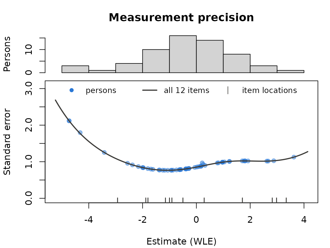
Polytomous and mixed tests
PP_gpcm() estimates abilities for the generalized
partial credit model. With all slopes equal to 1 (the default) this is
the partial credit model. thres has one column per item
with its thresholds; items with fewer categories have NA
below their last threshold. A first row of zeros is optional.
thres <- rbind(c(-1.5, -1, -0.5, 0, 0.5),
               c(0, 0.5, 1, 1.2, NA),
               c(1, 1.5, NA, 2, NA))
slopes <- c(1, 1.2, 0.8, 1.1, 0.9)
set.seed(1234)
x_gpcm <- sim_gpcm(thres = thres, alpha = slopes, theta = rnorm(200))
res_gpcm <- PP_gpcm(respm = x_gpcm, thres = thres, slopes = slopes, type = "wle")
head(res_gpcm$estimates)
#>      estimate        SE nsteps status
#> 1 -1.30077829 0.7936594      4     ok
#> 2 -0.09948067 0.6185704      4     ok
#> 3  1.87419642 0.6987634      3     ok
#> 4 -3.08511969 1.5519539      4     ok
#> 5  0.83380576 0.5892473      4     ok
#> 6 -0.74101448 0.6909744      4     ok
For a test with dichotomous and polytomous items, use
PPall(). Each column of thres holds the
thresholds of one item: a 4PL item has a single threshold (its
difficulty), a GPCM item has several, and this decides the model of each
item (findmodel() shows it). Lower and upper asymptotes
apply to the 4PL items only.
thres_mix <- rbind(c(-1, 0, 1, -0.5, 0.3),
                   c(NA, NA, NA, 0.6, 1.1))
findmodel(thres_mix)
#> [1] "4PL"  "4PL"  "4PL"  "GPCM" "GPCM"
x_mix <- sim_mixed(thres = thres_mix, alpha = c(1, 1.3, 0.9, 1, 1),
                   lowerA = c(0.2, 0.1, 0.15, 0, 0), theta = rnorm(200))
res_mix <- PPall(respm = x_mix, thres = thres_mix, slopes = c(1, 1.3, 0.9, 1, 1),
                 lowerA = c(0.2, 0.1, 0.15, 0, 0), type = "map")
summary(res_mix$estimates$estimate)
#>       Min.    1st Qu.     Median       Mean    3rd Qu.       Max.
#> -1.3044946 -0.4941779 -0.0471063 0.0009135 0.5158184 1.4540105sim_4pl(), sim_gpcm() and
sim_mixed() simulate responses for given item and person
parameters, as used above.
Jackknife
JKpp() leaves out each answered item once, estimates the
ability again and combines the pseudovalues into a jackknife estimate
and standard error (Wainer & Wright, 1980).
cmeth = "median" and cmeth = "AMT" (Andrews’
sine estimator) give robust estimates; the standard error is the same
for all three.
jk <- JKpp(res_wle)
head(jk$estimates)
#>     estimate        SE  L excluded status
#> 1 -0.9723726 0.6735435 12        0     ok
#> 2  1.8740917 0.6208916 12        0     ok
#> 3  1.0570466 0.4916653 12        0     ok
#> 4  1.5539111 1.6822352 12        0     ok
#> 5  0.3442215 0.5400380 11        0     ok
#> 6 -5.8298151 0.5859734 12        0     ok
head(JKpp(res_wle, cmeth = "AMT")$estimates)
#>     estimate        SE  L excluded status
#> 1 -0.3469704 0.6735435 12        0     ok
#> 2  1.3328207 0.6208916 12        0     ok
#> 3  1.0918816 0.4916653 12        0     ok
#> 4  2.0189363 1.6822352 12        0     ok
#> 5  0.7792898 0.5400380 11        0     ok
#> 6 -5.1186492 0.5859734 12        0     ok
Plausible values
Plausible values are draws from the posterior distribution of each
person. They need a prior, so PV() takes an estimate of
type "eap" or "map" and uses its prior (here
different for women and men).
set.seed(1)
pv <- PV(res_eap, npv = 5)
head(pv$pvdraws)
#>             PV1        PV2        PV3        PV4        PV5
#> [1,] -0.8002389 -0.3233673 -0.9233717  0.5076070 -0.2375027
#> [2,]  0.4360231  1.2839471  1.4466054  1.3412268  0.7699550
#> [3,]  1.6063897  0.8976006  0.2588440 -0.7478307  1.3619954
#> [4,]  0.4252652  0.4445135  1.0874052  1.0052948  0.8530677
#> [5,]  0.8941050  0.8083111  0.3646916 -0.9293031  0.7065487
#> [6,] -2.0791640 -2.1387964 -2.9255585 -2.3316668 -1.7955193
By default (approx = TRUE) the values are drawn from a
normal distribution with the posterior mean and standard deviation. With
approx = FALSE they are drawn from the posterior
itself.
References
Schuster, C., & Yuan, K. H. (2011). Robust estimation of latent ability in item response models. Journal of Educational and Behavioral Statistics, 36(6), 720–735.
Wainer, H., & Wright, B. D. (1980). Robust estimation of ability in the Rasch model. Psychometrika, 45(3), 373–391.
Warm, T. A. (1989). Weighted likelihood estimation of ability in item response theory. Psychometrika, 54, 427–450.